
Tilings and Projection Set Algorithms
Introduction
As part of my postdoctoral Miller fellowship, I have been developing computational imaging algorithms to recover the phase of an object from diffraction intensity measurements, using a technique called “electron ptychography”. One of the earliest and most successful algorithms for such phase retrieval is based on projection onto (non-)convex sets, which turns out to also be able to solve a variety of non-convex problems. Perhaps the most fun application is solving a Sudoku puzzle.
Sudoku Puzzles
Sudoku puzzles can be viewed as a constraint satisfaction problem, with the following well-known constraints:
- Each row contains only one of each of the numbers 1-9
- Each column contains only one of each of the numbers 1-9
- Each 3x3 ‘block’ contains only one of each of the numbers 1-9
- The solution must be consistent with a (minimum) set of pre-defined grid numbers
If we represent a Sudoku grid using a binary 9x9x9 array, where if the element \( Q\left(i,j,k \right) \) is equal to 1, then we place the number \( k \) on the \( \left(i,j\right) \) tile, then we can formalize these constraints as:
\[
\begin{align}
\sum_{k=1}^9 Q(i,j,k) &= 1 \quad \forall i,j \\
\sum_{i=1}^9 Q(i,j,k) &= 1 \quad \forall j,k \\
\sum_{j=1}^9 Q(i,j,k) &= 1 \quad \forall i,k \\
\sum_{i=1}^3 \sum_{j=1}^3 Q(i+U,j+V,k) &= 1 \quad \forall k \text{ and } \; U,V \in \left\{ 0,3,6 \right \} \\
Q(i,j,:) &= \gamma_{i,j} \quad \forall i,j \in J',
\end{align}
\]
where \(
\gamma_{i,j} \) is the unit-vector representing the known symbols in \(
J'\).
Note that the first constraint, namely that the sum over the vector of symbols must equal 1 for each tile, combined with the fact that our representation only allows binary values of 0 or 1, ensures we have a single symbol at each cell.
As formulated above, the problem lends itself well to Linear Programming solutions, e.g. the SolveSudokuPuzzle resource function, which has the minimal source code:
SolveSudokuPuzzle[known_SparseArray] := Module[{z,sudokuConstraints,vars,knownConstraints,res,i,j,k,l,n,m=Length[known]},
  n = Sqrt[m];
  sudokuConstraints={
    Table[{Total[z[i,j]]==1,0\[VectorLessEqual]z[i,j]\[VectorLessEqual]1,z[i,j]\[Element]Vectors[m,Integers]},{i,m},{j,m}],
    Table[{Sum[z[i,j],{j,m}]==1,Sum[z[j,i],{j,m}]==1},{i,m}],
    Table[Sum[z[i+k,j+l],{k,m},{l,m}]==1,{i,0,m-n,n},{j,0,m-n,n}]
  };
  knownConstraints=MapThread[Indexed[z@@#1,Abs[#2]]==If[#2<0,0,1]&,{known["NonzeroPositions"],known["NonzeroValues"]}];
  vars=Flatten[Table[z[i,j],{i,m},{j,m}]];
  LinearOptimization[0,{sudokuConstraints,knownConstraints},vars]
]
Back to projection set algorithms, Veit Elser and co-authors showed that the Sudoku constraints can be interpreted as projection operators to appropriate non-convex sets and solved using a specific projection set algorithm called the “difference map” algorithm. We will skip most of the implementation details, but as an example the single-symbol constraint for each tile can be implemented as a projection operator which sets the maximum-value index to 1 and the rest of the elements of the vector to zero, i.e.:
projectToUnitVector[vector_]:=UnitVector[9,First@FirstPosition[vector,Max[vector],{1},Heads->False]]
squareProjection[array_]:=Map[projectToUnitVector,array,{2}]
Here’s a fun online demo of the projection sets algorithm at work solving Sudoku puzzles. For more information, see this wonderfully-clear thesis on the topic.
Constrained Tilings
Considering the sets satisfying the above 5 constraints are highly non-convex, I was curious to see if projection set algorithms could solve another favorite problem of mine which can be formulated using linear constraints, namely that of constrained tilings.
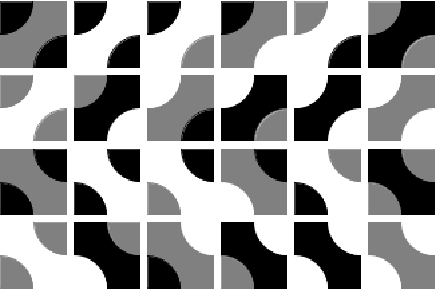
The problem is formulated as follows: given an \( \left(n,m\right) \) target image, and a set of \( L \) (colored) tiles, find the arrangement of tiles which most closely approximates the target image’s color values, while respecting the topological constraints between adjacent tiles. For example, in the set of 24 grayscale “Smith” tiles shown below, the tiles in the first two rows in the third column are allowed to be placed on top of each other, but the tiles in the first two rows of the first column are not.
For the sake of brevity, we once again omit most implementation details, but briefly the projections are given by:
- Similar to the Sudoku puzzles, we represent our tiling using an \( \left(n,m,L\right) \) array and only allow one tile per pixel. As such, the first constraint and thus projection operator is the same as above.
- The target-image-constistency constraint we choose is also fairly straightforward: we simply weigh the current iteration vector at each pixel according to a Gaussian kernel centered on the tile’s color value minus the target image color value at that pixel.
- The tiling constraint projection is perhaps less obvious. Denote the set of \( M \) topological constraints acting on a vectorized version of our array \( \vec{x} = \text{vec}\left(Q(i,j,t)\right) \), using the \( \left(M,n \times m \times L\right) \) matrix \( C \), such that \( C \cdot \vec{x} = 0 \). The orthogonal projector onto the nullspace of the topological constraints is therefore given by: \[ P_{C}(\vec{x}) = \left(\mathbb{I} - C^+\cdot C \right)\cdot \vec{x}, \] where \( C^+ \) denotes the Moore-Penrose pseudoinverse of the topological constraints matrix.
We implement these three projections using the “relax-reflect-reflect” algorithm (a variant of the “difference-map” algorithm, with a tunable step-size) and, lo and behold, it works!
I hope you find watching the algorithm trying to climb out of a local minimum as mesmerizing as I do! If you are curious about the source code, here is a cloud notebook.