Counting Digits of Pi
Introduction
As part of the MIT course 3.029 I taught in the spring of 2022, we held optional coding “get-togethers” once a week, alternating between “Data-Visualization Hour” and “Code Show and Tell”. In particular, the week of Pi day happened to fall on “Code Show and Tell” and the students thought it’d be fun to code up one of the craziest Pi-related phenomena I know.
This is very beautifully explained in the 3Blue1Brown video below:
Mathematica SE solution
First, note that this exact question was asked on the Mathematica SE in 2020 - with a very natural numeric solution using DiscreteVariables in NDSolveValue.
numericSolution[d_] := Module[{
   collisions = 0, m1 = 1, m2 = 100^(d - 1),
   x10 = 1, x20 = 2, v10 = 0, v20 = -1, tmax = 20,
   etot, newvelocity, vsol, sol
   },

  etot = m1 v10^2 + m2 v20^2;
  newvelocity[vv1_, vv2_] := Block[{tsol},
    tsol =
     Quiet[Solve[{m1 vn1 + m2 vn2 == m1 vv1 + m2 vv2,
        m1 vn1^2 + m2 vn2^2 == etot}, {vn1, vn2}]]; {vn1, vn2} /.
     If[Sign[tsol[[1, 1, 2]]] != Sign[vv1], tsol[[1]], tsol[[2]]]
    ];

  sol = NDSolveValue[{
     x1'[t] == v1[t], x2'[t] == v2[t],
     x1[0] == x10, x2[0] == x20, v1[0] == v10, v2[0] == v20,
     WhenEvent[x1[t] == x2[t], {
       collisions += 1,
       vsol = newvelocity[v1[t], v2[t]],
       v1[t] -> vsol[[1]],
       v2[t] -> vsol[[2]]
       }],
     WhenEvent[x1[t] == 0, {
       collisions += 1,
       v1[t] -> -v1[t]
       }]},
    {x1, x2, v1, v2}, {t, 0, tmax}, DiscreteVariables -> {v1, v2}];
  Echo[collisions];
  sol
  ]
Event-Based Elastic Collisions
It’s instructive however to code this up from scratch using simple elastic collisions!
Collision Times
Consider the collison between two particles, assumed to be a distance \( 2r \) apart. The trajectories of the two particles can be computed using their positions, instantaneous velocities, and time:
trajectory1  = x1 + v1 t;
trajectory2 = (x1 + Δx) + (v1 + Δv) t;
Their separation squared is therefore given by:
separationSquared =
 Simplify[With[{delta = trajectory2 - trajectory1}, delta . delta]]
The Wolfram Language makes no assumptions about the dot products since we’ve kept all our variables symbolic, so let’s help it out a bit by introducing simple multiplication rules:
separationSquared = Distribute[separationSquared] //. {
   ( t a_ ) . ( t b_ ) :> t^2 a . b,
   ( a_ ) . ( t b_ ) :>  t a . b ,
   ( t a_ ) . ( b_ ) :>  t a . b,
   ( Δv . Δx ) :> ( Δx . Δv )
   }
We’re now ready to find the collision times, i.e. the times \( t \) when the expression for the squared distance above equals \( 4r^2 \).
{firstCollision, secondCollision} =
 t /. Simplify[Solve[separationSquared == (2 r)^2, t]]
Note that since our equation is quadratic in time, there are two collision solutions. It’s probably easiest to show their difference graphically using an example:
We’re interested in the first collision time, when the particles first touch: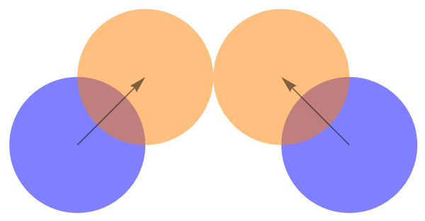
The second collision time corresponds to the time the particles have separated again post-collision, had they been allowed to pass straight through each other: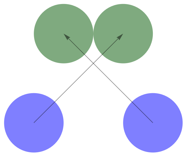
We can now write a function which returns the collision time:
particleParticleCollisionTime[{p1 : {m1_, x1_, v1_}, p2 : {m2_, x2_, v2_}}] :=
 Block[{dummyMass, dx, dv, dxdv, dvdv, dxdx, rootTerm},

  {dummyMass, dx, dv} = p2 - p1;
  dxdv = dx . dv;

  If[dxdv >=  0, Return[\[Infinity]]];

  dxdx = dx . dx;
  dvdv = dv . dv;
  rootTerm = dxdv^2 + (dvdv (1 - dxdx));

  If[rootTerm < 0, Return[\[Infinity]]];

  -(dxdv + Sqrt[rootTerm])/dvdv
  ]
Note that we’ve assumed the particles have a radius \(
r=1/2 \) for simplicity and instructed our function to return Infinity if our particles are moving away from each other and will not collide.
This allows us to write a simple function to return the position of particles at time \( t \):
particleStateAtTime[particle : {m_, x_, v_}, time_] := {m, x + time v, v}
Velocities Post-Collision
The velocities post-collision are given using energy and momentum conservation:
conservationLaws[1] = {
   m[1] u[1] + m[2] u[2] == m[1] v[1] + m[2] v[2],
   1/2 m[1] u[1]^2 + 1/2 m[2] u[2]^2 ==
    1/2 m[1] v[1]^2 + 1/2 m[2] v[2]^2
   };
Solve[conservationLaws[1], {v[1], v[2]}]
This generalizes nicely to higher dimensions:
bounceVelocitiesAfterCollision[{p1 : {m1_, x1_, v1_}, p2 : {m2_, x2_, v2_}}] :=
 Block[{dv = v2 - v1, dx = x2 - x1, deltaV, \[Mu] = m1 m2/(m1 + m2), \[Delta]v},

  \[Delta]v = (dv . dx (dx))/dx . dx;
  {
   {m1, x1, v1 + (2 \[Mu])/m1 \[Delta]v},
   {m2, x2, v2 - (2 \[Mu])/m2 \[Delta]v}
  }
 ]
It would be convenient if we could treat particle-wall collisions using our existing framework.
To do so, we consider an “immovable” wall as a stationary object with Infinite mass.
This requires we specialize our two functions above using pattern matching (mathematica’s analogue of multiple dispatch):
bounceVelocitiesAfterCollision[{p1 : {\[Infinity], x1_, v1_},
   p2 : {m2_, x2_, v2_}}] :=

 Block[{dv = v2, dx = x2 - x1, deltaV, \[Delta]v},
  \[Delta]v = (dv . dx (dx))/dx . dx;
  {
   {\[Infinity], x1, v1},
   {m2, x2, v2 - 2 \[Delta]v}
   }
  ]

bounceVelocitiesAfterCollision[{p1 : {m1_, x1_, v1_},
   p2 : {\[Infinity], x2_, v2_}}] :=

 Block[{dv = -v1, dx = x2 - x1, deltaV, \[Delta]v},
  \[Delta]v = (dv . dx (dx))/dx . dx;
  {
   {m1, x1, v1 + 2 \[Delta]v},
   {\[Infinity], x2, v2}
   }
  ]
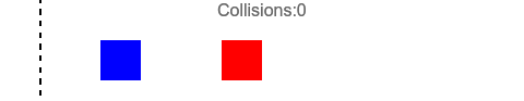
Colliding Blocks Setup
As we alluded to above, we’ll consider three “blocks”:
- An “immovable” rigid block (wall) at \( x = \{-1/2\} \)
- An initially stationary (blue) block with \( m = 1 \), at \( x = \{2\} \)
- A (red) block with \( m = 100^{d-1} \), at \( x = \{5\} \), moving to the left with \( v = \{-1\} \)
particleStates[d_] := {
  {\[Infinity], {-1/2}, {0}},
  {1, {2}, {0}},
  {100^(d - 1), {5}, {-1}}
  }
As such, we have two possible collisions to consider:
- Blue block colliding with the wall
- Blue block colliding with the red block
At each iteration, we will:
- Compute the two possible collision times
- Pick the smallest time
- Update the positions and velocities post-collision
- Rinse and repeat
findShortestCollisionTime[{t_, particleStates : {wall_, blue_, red_}}] :=
 Block[{wallBlue, blueRed},
  wallBlue = particleParticleCollisionTime[{wall, blue}];
  blueRed = particleParticleCollisionTime[{blue, red}];
  {Min[{wallBlue, blueRed}], Ordering[{wallBlue, blueRed}]}
  ]

bounceParticlesAtShortestCollision[{t_, particleStates : {wall_, blue_, red_}}] :=
 Block[{time, ordering, preWall, preBlue, preRed, post},

  {time, ordering} = findShortestCollisionTime[{t, particleStates}];
  If[time == \[Infinity], Return[{t, particleStates}]];

  {preWall, preBlue, preRed} = particleStateAtTime[#, time] & /@ particleStates;

  post = Switch[ordering,
    {1, 2},
    Append[bounceVelocitiesAfterCollision[{preWall, preBlue}], preRed],
    {2, 1},
    Prepend[bounceVelocitiesAfterCollision[{preBlue, preRed}], preWall]
    ];

  {t + time, post}
  ]
The ‘do-nothing’ clause inside our function above, ensures that if both collision times are Infinity, then the particle state returns unchanged.
This allows us to use FixedPointList to conveniently exhaust the simulation until both our blocks fly away towards the right, terminating the simulation:
eventsList[digits_] :=
 N[Most[FixedPointList[
    bounceParticlesAtShortestCollision, {0, N[particleStates[digits]]}]]]
Visualization Functions
Finally, we write two utility functions to build a linear interpolation on the blocks’ positions given our collisions event list:
positionsInterpolator[listOfEvents_] := With[{
  times = listOfEvents[[All, 1]],
  positions1D = Transpose[listOfEvents[[All, 2, All, 2, 1]]]
  },
  Table[Interpolation[Transpose[N[{times, positions}]],
    InterpolationOrder -> 1], {positions, positions1D}]
 ]

visualizeBlocks[t_, times_][{wall_InterpolatingFunction,
   blue_InterpolatingFunction, red_InterpolatingFunction}] :=

 Graphics[{
   {EdgeForm[Directive[Black, Dashed]], FaceForm[None],
    Rectangle[{-10, -10}, {0, 10}]},
   {Blue, Rectangle[{blue[t] - 1/2, -1/2}, {blue[t] + 1/2, 1/2}]},
   {Red, Rectangle[{red[t] - 1/2, -1/2}, {red[t] + 1/2, 1/2}]}
   }, PlotRange -> {{-1, 12}, {-1, 1}},
  PlotLabel ->
   StringTemplate["Collisions:`1`"][
    First[FirstPosition[times, ts_ /; ts > t, {Length[times] + 1}]] -
     2]
  ]
Animation
We can wrap everything together to produce animations of the sort:
Module[{
  events = eventsList[3],
  interpolators, times
  },
 times = events[[All, 1]];
 interpolators = positionsInterpolator[events];
 Animate[visualizeBlocks[t, times][interpolators], {{t, 0, "Time"}, 0,
    Last[times]}, AnimationRepetitions -> 1, Paneled -> False,
  AnimationRunning -> False]
 ]